In this post we cover two papers that apply topological deep learning to three flavors of representation learning: autoencoders, self-supervised learning, and metric learning. It is recommended to read the previous post before this one.
General setup
Encoder
The goal of representation learning in the non-manifold setting is learning an encoder $f: \mathcal{X} \to \mathbb R^d$, where $\mathcal{X}$ is the dataset and $d$ is the desired dimension of the representation. Typically $f$ will be a neural network, whose weights are learned.
In our setup, we want to change the target space $\mathbb R^d$ to one that is more topologically interesting. We do this by learning an atlas of $\mathcal X$ comprised of $k$-many charts, each one being a mapping
$$\phi_i: \mathcal{X} \to \mathbb R^d, ~~ i=1, \ldots, k$$
Each chart is typically defined on an open subset of the manifold and we introduce the function $$ q = (q_1, \ldots, q_k): \mathcal{X} \to [0, 1]^k $$ that provides chart membership: $q_i(x) \approx 1$ when $x$ belongs to chart $i$. In other words, we can think of $q_i$ as a probability distribution for membership of chart $i$.
We will see that we can typically get away with much smaller $d$ than we would in the classical, Euclidean setup. This is a significant benefit because of the benefit data compression and avoiding phenomena involving the curse of dimensionality.
Measuring distances
Some algorithms require defining a distance on either the embedding space or $\mathcal{X}$ itself. In our atlas setting we form a metric by taking the standard Euclidean distance in the charts and then weighing by the chart membership function $q$ if the points have a non-zero probability of being in a common chart. If not, then the distance between them is infinite. Explicitly: $$ d_{q, \phi}(x, y) = \begin{cases} \frac{\sum_i q_i(x) q_i(y) || \phi_i(x) - \phi_j(x) ||}{\sum_i q_i(x) q_i(y)}; \text{ if $\sum_i q_i(x) q_i(y) \ne 0$.}\\ \infty; \text{ otherwise} \end{cases} $$
Statistical model and regularization
We find it useful to take a latent variable model perspective. Here, the latent space is
$$ \mathcal Z = \{1, \ldots, k\} \times [0, 1]^d $$ and we will use $X, J, Z$ to denote random variables on the spaces $\mathcal X$, $\{1, \ldots, k\}$, and $[0,1]^d$, respectively. Thus the goal of $q_i(x)$ is to match $p(J=i | X =x)$.
Regualization on the embedding space then becomes prescribing a prior distribution $\mathcal Z$, which we take be the uniform distribution, $\operatorname U(\mathcal Z)$. Additionally, we add a regularization term to $q$ to encourage it to be a deterministic distribution for a given point, i.e. that for most $x \in \mathcal X$, $q_i(x) \approx p(J=i | X=x)$ should be low entropy. This is critical because if $q_i(x)$ were say uniform in $i$ then we would not be able to faithfully represent $x$ as an element in a single chart, thus essentially representing points as living in the union of charts, $\mathbb R^{d \times k}$, defeating the entire purpose of learning a condensed representation.
Autoencoders
Setup
In our paper we apply this general framework to autoencoders, and in particular modify Wasserstein Autoencoders (WAEs) , which are generalizations of Adversarial Autoencoders (AAEs) , to work in the manifold setting.
Autoencoders (in constrast to contrastive and metric learning, which we cover in the next sections) have a generative component to them: a mapping from the latent/embedding space back to the original space. In our manifold setting the latent space is the atlas $[0, 1]^d \times \{0, \ldots, k\}$ and so besides the maps $\phi_i: \mathcal X \to \mathbb [0,1]^d$ we also learn the inverse maps $\psi_i: [0,1]^d \to \mathcal X$.
The goal of WAEs is to match the distribution on the entire latent space to a prior, which constrasts with variational autoencoders which have the goal of matching the distribution of the latent space conditioned on a point $x \in \mathcal X$ to match a prior. For manifolds, this is exactly what we want since the distrubiton on charts can be prescribed to be uniform. Further, WAEs allow deterministic encoders and decoders, which is what we will use.
Unpacking the objective of WAE in the manifold setup gives us the loss function $$ \frac{1}{N} \sum_{i=1}^N q_j(x_i) || x_i - \psi_j(\phi_j(x_i)) ||^2 + \lambda \operatorname{JS}\left((\phi \times q)_* \mathcal X, \operatorname U (\mathcal Z)\right), $$ where the first term is the reconstruction loss (on a collection of random samples $x_i \in \mathcal X$) and the second term is the Jensen-Shannon divergence between the uniform distribution and the distribution on the latent space coming from the encoder, which we use a GAN objective for (recall that the GAN objective is precisely the minimization of Jensen-Shannon divergence), viewing the encoder as the generator.
Data viz
One of the nice things we get from this is both dimensionality reduction (the maps $\phi_i$) and a “fuzzy” clustering of the data (via $q$). Here “fuzzy” refers to the fact that clustering is soft, in terms of $q(x)$ assigning a probability of of $x$ belonging to cluster $i$ (with this distribution being skewed towards a single chart for most $x$). We can use this define intersections of charts (and intersections of intersections).
For example, in the case of two charts we can use $q$ to define a measure of how much they overlap. Namely, $\mathbb E_{x \sim p(X | J = j_0)} p(J = j_1 | X = x)$ is a measure of how much chart $j_0$ is a subset of $j_1$. Then we can define the strength of interesection between two charts as
$$ u_{j_0 j_1} = \frac{1}{2}\left(\mathbb E_{x \sim p(X | J = j_0)} p(J = j_1 | X = x) + \mathbb E_{x \sim p(X | J = j_1)} p(J = j_0 | X = x) \right) $$ which can be approximated using a random sample $x_1, \ldots, x_n \in \mathcal X$ as
$$ u_{j_0 j_1} \approx \left(\frac{1}{\sum_i q_{j_0}(x_i)} + \frac{1}{\sum_i q_{j_1}(x_i)}\right) \sum_{i=1}^N q_0(x_i) q_1(x_i) $$
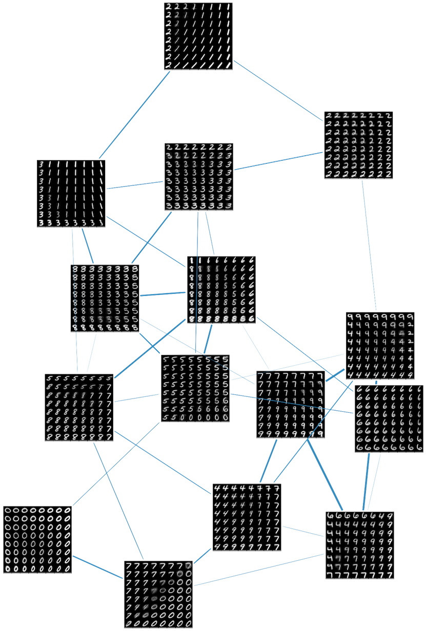
For a nice visualization, we train such an autoencoder to fit MNIST using $d=2$ and $k=15$. We take a uniform grid of points on each chart (the unit square in this case) and then use the decoder to generate elements of MNIST, giving fifteen grids of images. We then draw a line between them that is weighted by $u_{j_0 j_1}$. From the image we see solid clustering of the data by digit as well as strong overlaps between charts that have similar looking digits.
The fuzzy Čech nerve
Note: this section is a bit more mathematically involved; feel free to skip ahead →
The definition of $u_{j_0 j_1}$ can be bootstrapped to define the intersection strength of an arbitrary number of charts, providing a collection of elements ${u_{j_0 \ldots j_k}} \subset (0, 1)$. For the mathematically minded, this can be thought of as a fuzzy Čech nerve of the space $\mathcal X$. Further, we can borrow from the playbook of Topological data analysis (TDA) and introduce a parameter $\varepsilon > 0$. Fixing $\varepsilon$ and thresholding the $u_{j_0 \ldots j_k}$ by it gives a (regular) simplicial complex, which we can compute the homology of (and recall the beautiful fact that for good covers the simplicial homology of the Čech nerve is the same as the homology of the underlying topological space). By varying $\varepsilon$ we then get a graph, analgous to the barcodes of TDA, of the persistence of the homology groups. In the paper we did an experiment on this for $\mathbb RP^2$ (which we recall has $H_1(\mathbb RP^2) = \mathbb Z / 2$), which gave the following
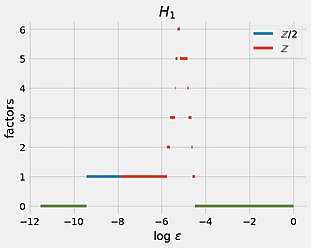
In the paper we also discuss a simpler method for defining overlaps for a given $\epsilon$, which actually gave a more accurate barcode in this case.
Intrinsic dimensionality estimation
A problem with dimensionality reduction algorithms is: how do you choose $d$ or know that you picked the right value for it? If its too small then you lose the information contained in the dataset while its too large you get less out of dimensionality reduction than you could. In the machine learning literature, the ideal value is typically called the datasets instrinsic dimension, which we will denote by $d^*$. We looked into how good our autoencoding algorithm is at gauging whether the choice of $d$ used is in the right ballpark of the intrinsic dimension.
The idea is to look at the reconstruction loss and GAN loss of the encoder during training. Recall that in the GAN loss (confusingly) for WAE/AAEs, the encoder is the generator since the GAN training is happening on the latent space, and the encoder therefore is trying to make it impossible for the discriminator to detect whether an element was generated by the encoder or randomly sampled from the latent space. In the ideal, this loss should be $\log 2 \approx 0.69$, which means the discriminator is essentially flipping a coin to determine what is sampled versus generated.
The bigger $d$ is, the easier it is to exactly reconstruct an input since there is no significant bottleneck, but if $d \gg d^*$ then the encoder will be mapping a lower dimensional object into a higher-dimensional one, which makes the discriminator’s job easy and therefore the GAN loss of the encoder will be high. On the other hand, if $d \ll d^*$ it will be easy to trick the discriminator (projecting from a high dimensional space to look like a lower dimensional one is simple) but the reconstruction loss will be high. Therefore, good values of $d$ correlate (no surprise) to both components of the overall loss being ideal: the reconstruction loss low and the GAN loss close to $\log 2$.
We did a simple experiment by generating data on the 3-torus $\mathbb T^3 = S^1 \times S^1 \times S^1$ embedded into $\mathbb R^6$ using the standard embedding of the circle $S^1$ into $\mathbb R^2$. Then we trained manifold autoencoders with dimensions $d=1, 2, \ldots, 5$ and plotted the loss curves.
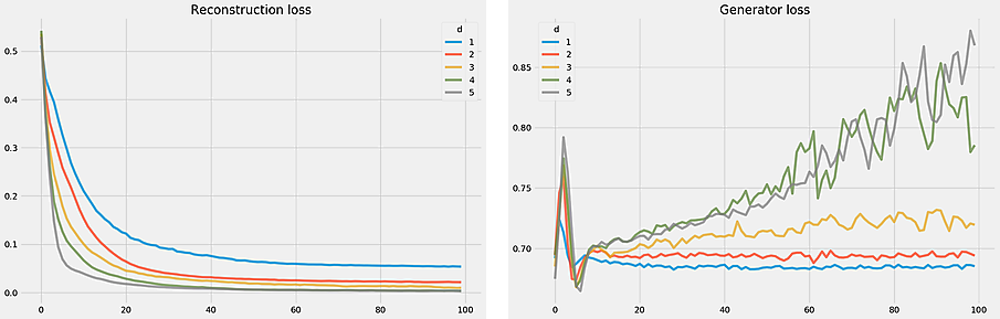
While it’s not clear that $d=3$ (which is the actual intrinsic dimension) wins here over $d=2$, we do see the anticipated trends at play.
Contrastive and metric learning
In our newest work we apply our manifold approach to both constrastive learning (in particular SimCLR ) and metric learning, mostly focusing on low dimensions (up to $d=8$). We keep the same atlas framework of the previous paper except we change how we regularize the latent space to be uniform: instead of the GAN-based technique we now use a maximum mean discrepancy (MMD) loss (which is a variant that the WAE paper does too). This simplifies the training since we do not need a discriminator network and the objective is much more stable. Code for the experiments discussed in this section can be found in this repo .
Manifold based SimCLR
SimCLR is a simple technique to learn useful representations of image data (though the idea could be applied to any dataset where you can easily compute data augmentations) in a completely unsupervised way. The goal is to learn a lower-dimensional representation of the dataset such that the distance between similar images is small and the distance between disimilar ones is large. In this unsupervised setting we do not have labels that we can use to determine groundtruth similarity, so instead we choose a set of augmentations $A = {a_1, \ldots, a_\ell}$, each one a map $\mathcal X \to \mathcal X$ and then train on the augmented dataset, with an objective for encourage $a_1(x)$ and $a_2(y)$ to be close together if and only if $x = y$. The augmentations used are just random crop-and-resize, and random horizontal flip.
Interestingly, the paper finds that you get better performance not by using the contrastive loss on the embedding space directly but instead on an auxillary projection head. Formally, let $f : \mathcal X \to \mathbb R^d$ be the embedding function to be learned. Then we add a new learnable network head $h :\mathbb R^d \to \mathbb R^{\tilde d}$ (where typicall $\tilde d < d$). During training the contrastive loss operates on $h \circ f$, while during inference $h$ is dropped.
To adjust this to our manifold approach, which we call MSimCLR we replace learning $f$ with learning an atlas $(q, \phi_1, \ldots, \phi_k)$, and introduce projection heads on each chart: $h_1, \ldots, h_k$. During training, we produce a single vector in the projection space by taking a sum of the projections weighted by $q$, i.e. using the map $$ \mathcal X \to \mathbb R^{\tilde d}, ~~ x \mapsto \sum_i q_i(x) h_i(\phi_i(x)) $$ We then train this against the exact same loss that vanilla SimCLR uses.
The evaluation process that the SimCLR paper uses is to run SimCLR on a classification dataset (we will use MNIST, FashionMNIST, and CIFAR10), train a linear classifier from the embedding space $\mathbb R^d$ on a train dataset, and then compute the classification accuracy on the test data. A global linear classifier does not make sense in our manifold setting so we add a linear network $L_i:[0,1]^d \to [0,1]^c$ on each chart, where $c$ is the number of classes. Then for any point in the dataset, we use the linear classifier on the chart it is most likely to belong to, i.e. the logits associated to a point $x \in \mathcal X$ are $L_{i^*}(\phi_{i^*}(x))$ where $i^* = \argmax_i q_i(x)$.
Our results are summarized in the following table
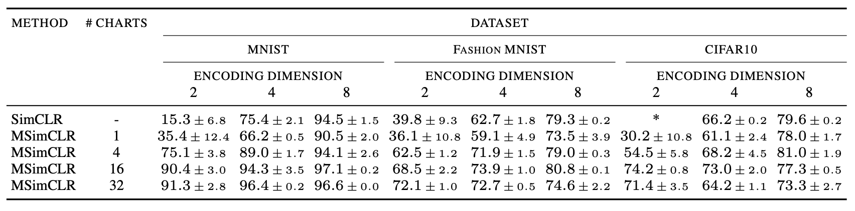
Evaluation accuracy. The * denotes that we were not able to get a model to converge when training.
The punchlines
Low-dimensional SimCLR beats SimCLR out of the water. This means in particular that we get very nice and accurate data visualizations in two-dimensions (see the appendices of the paper for examples). Also very interesting is the row with #charts = 1. In this case, MSimCLR is just SimCLR augmented by the MMD regularization loss on the embedding space. In dimension two this added regularization alone drastically improved SimCLR’s performance in the case of MNIST and CIFAR10 (the latter of which was impossible to train without it). We will see a similar phenonema in the metric learning section but in high dimensions.
Manifold based triplet training
Next we turn to metric learning. In metric learning we have a collection of labeled data, with the goal of learning an embedding map such that objects of the same class are close together. The classic use case for this is in face recognition, where you have an annotated training dataset consisting of a handful of face images for a given person.
For our manifold setup we use the standard triplet loss training and the distance function defined in this section above . We evaluate on the standard metric learning benchmarks datasets CUB-200 and Standford Cars using the standard recall@n (R@n) metric. Our results, compared to vanilla triplet loss training, are:
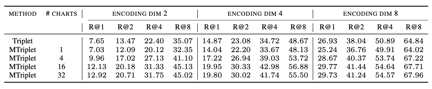
CUB-200
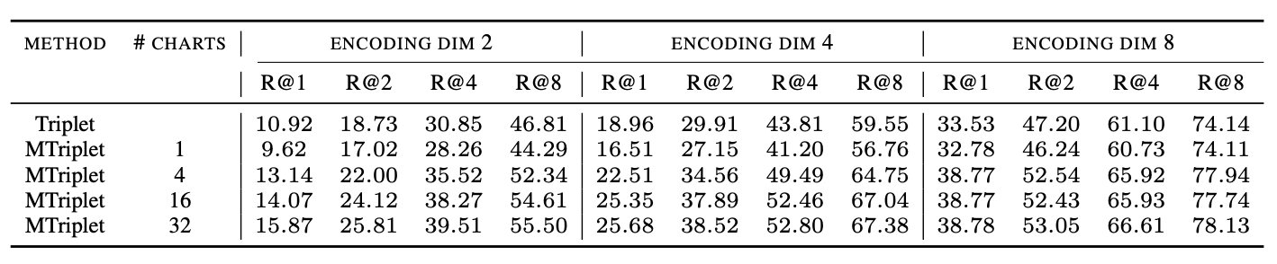
Standford Cars
Again, just like for SimCLR, we see that the manifold approach clearly wins in low dimensions.
Regularization alone significantly improves performance in higher dimensions
Perhaps the most interesting thing to come out of this was something that actually does not have much to do with manifolds. Note that, unlike for SimCLR, we do not see that just adding MMD-based regularization to standard triplet training (i.e. the row #charts = 1 row) helps for these small dimensions. However, we did an experiment in 64-dimensions (a more common choice of dimension for metric learning) and found very suprisingly that just adding the MMD regularization to vanilla triplet training gives a huge performance boost. Below are plots for R@1 on the test set versus training epoch
R@1 for CUB-200 R@1 for Stanford Cars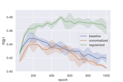
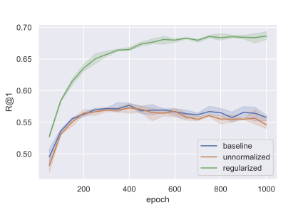
Here, “baseline” is standard triplet training (which normalizes vectors), “unnormalized” is standard triplet training but without the normalization (this is to isolate the MMD-contribution since in our manifold setting we do not unit-normalize vectors), and “regularized” is just “unnormalized” with MMD-regularization (i.e. our manifold setup with just a singel chart).
Potential application: Vector databases
We highlight one potential practical application to be explored here. Vector databases have been booming recently, but the larger the dimension of the vectors, the more memory required and the slower the queries are. Our results show that we can obtain massive compression without sacrificing significant information by fitting a very low-dimensional manifold to the data. Then in the vector database, for every point $x$ one would store $\argmax_i q_i(x)$ (which is just a couple bits of information) and $\phi_{\argmax_i q_i(x)}(x) \in [0,1]^d$. This would be useful for resource constrained systems, such as edge devices, or any situation where one is willing to sacrifice a bit of recall accuracy in order to boost query speed.